Tutorial¶

Import the DAS4Whales module and dependencies from GitHub¶

If not in a Jupyter notebook, follow the Installation instructions, otherwise, run the following cell to install the module

!python3 -m pip install das4whales

Import the DAS4Whales module and dependencies for the example¶

import das4whales as dw
import scipy.signal as sp
import numpy as np

Download some DAS data¶

Here, we check if the file stored at the chosen url already exists otherwise we download a .hdf5 file from the OOI DAS experiment (Wilcock & OOI, 2023). The file is ~850 MB so the download might take a few seconds.

Experiment information can be found on the OOI website.

# The dataset of this example is constituted of 60s time series along  66 km of cable
url = 'http://piweb.ooirsn.uw.edu/das/data/Optasense/NorthCable/TransmitFiber/' \
        'North-C1-LR-P1kHz-GL50m-Sp2m-FS200Hz_2021-11-03T15_06_51-0700/'\
        'North-C1-LR-P1kHz-GL50m-Sp2m-FS200Hz_2021-11-04T020002Z.h5'

filepath, filename = dw.data_handle.dl_file(url)

North-C1-LR-P1kHz-GL50m-Sp2m-FS200Hz_2021-11-04T020002Z.h5 already stored locally

Get information on the DAS data from the hdf5 metadata¶

By reading a hdf5 file’s metadata, we can access the acquisition parameters, without loading the associated “big” strain data matrix. In the perspective of looping through several files and in the interest of speed & repeatability, this enables us to select the desired channels and design appropriate filters once and for all.

Note: the metadata reading function das4whales.data_handle.get_acquisition_parameters(params) is prepared to read the metadata recorded by an OptaSense interrogator. This function will likely need to be adapted for different metadata format, e.g., collected by a different model of interrogator.

# Read HDF5 files and access metadata
# Get the acquisition parameters for the data folder and store them in a dictionary
metadata = dw.data_handle.get_acquisition_parameters(filepath, interrogator='optasense')
fs, dx, nx, ns, gauge_length, scale_factor = metadata["fs"], metadata["dx"], metadata["nx"], metadata["ns"], metadata["GL"], metadata["scale_factor"]

print(f'Sampling frequency: {metadata["fs"]} Hz')
print(f'Channel spacing: {metadata["dx"]} m')
print(f'Gauge length: {metadata["GL"]} m')
print(f'File duration: {metadata["ns"] / metadata["fs"]} s')
print(f'Cable max distance: {metadata["nx"] * metadata["dx"]/1e3:.1f} km')
print(f'Number of channels: {metadata["nx"]}')
print(f'Number of time samples: {metadata["ns"]}')

Sampling frequency: 200.0 Hz
Channel spacing: 2.0419046878814697 m
Gauge length: 51.0476188659668 m
File duration: 60.0 s
Cable max distance: 66.6 km
Number of channels: 32600
Number of time samples: 12000

Select the desired channels and channel interval¶

As displayed above, the channel spacing (spatial sampling all along the fiber) is very narrow, close to 2 m. The following allows to re-sample the data spatially and select a region of interest, in the interest of minimizing the matrix’s size.

Warning

Depending on the RAM available on your computer, you may need to adjust (lower) the number of channels selected and the channel interval.

selected_channels_m = [20000, 65000, 10]  # list of values in meters corresponding to the starting,
                                          # ending and step wanted channels along the FO Cable
                                          # selected_channels_m = [ChannelStart_m, ChannelStop_m, ChannelStep_m]
                                          # in meters

selected_channels = [int(selected_channels_m // dx) for selected_channels_m in
                     selected_channels_m]  # list of values in channel number (spatial sample) corresponding to the starting, ending and step wanted
                                           # channels along the FO Cable
                                           # selected_channels = [ChannelStart, ChannelStop, ChannelStep] in channel
                                           # numbers

print('Begin channel #:', selected_channels[0], 
      ', End channel #: ',selected_channels[1], 
      ', step: ',selected_channels[2], 
      'equivalent to ',selected_channels[2]*dx,' m')

Begin channel #: 9794 , End channel #:  31833 , step:  4 equivalent to  8.167618751525879  m

Create the filters to condition the data¶

The module das4whale.dsp (where dsp stands for digital signal processing) is written in a way that allows filters design before application. This choice was made to make the processing a large number of files more efficient by avoiding recalculating the filters.

Here the filters are set to preserve fin whale 20-Hz song, present in most of the dataset, see:

Wilcock, W. S., Abadi, S., & Lipovsky, B. P. (2023). Distributed acoustic sensing recordings of low-frequency whale calls and ship noise offshore Central Oregon. JASA Express Letters, 3(2), 026002. DOI: https://doi.org/10.1121/10.0017104

# Create band-pass filter for the TX plots
sos_bpfilter = dw.dsp.butterworth_filter([5, [10, 30], 'bp'], fs)

# Create high-pass filter
sos_hpfilter = dw.dsp.butterworth_filter([2, 5, 'hp'], fs)

Load raw DAS data¶

Loads the data using the pre-defined selected channels.

# Load DAS data
tr, time, dist, fileBeginTimeUTC = dw.data_handle.load_das_data(filepath, selected_channels, metadata)

Apply band-pass filter and corresponding t-x plot¶

# band-pass filter
trf = sp.sosfiltfilt(sos_bpfilter, tr, axis=1)

# Plot
dw.plot.plot_tx(sp.hilbert(trf, axis=1), time, dist, fileBeginTimeUTC, fig_size=(12, 10), v_min=0, v_max=0.4)

png

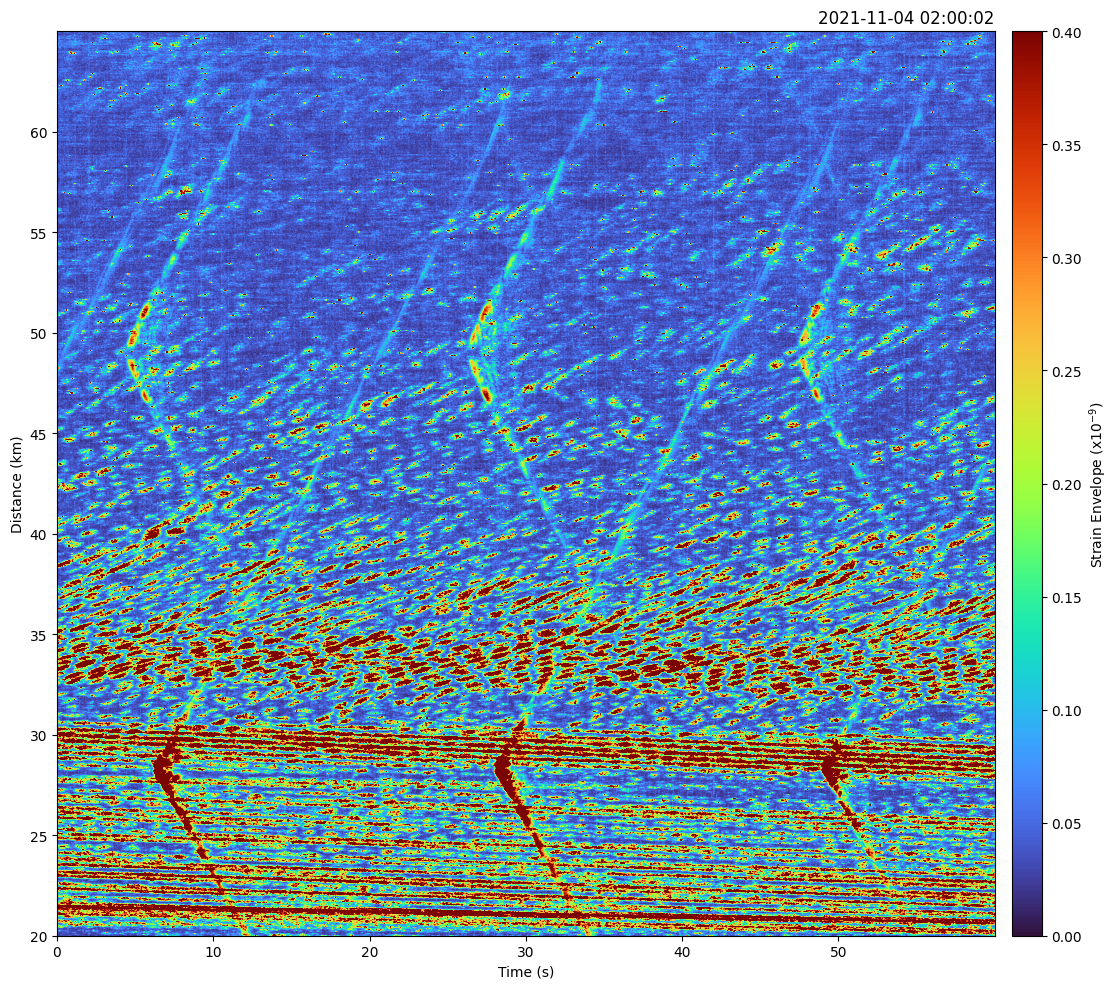
The spatio-temporal plot (t-x plot) shows temporal variations of the strain along the fiber optic cable between 20 and 65 km, every 8.17 m corresponding to the selected channels. We observe signals emitted by punctual sources and propagating close to the underwater sound speed, with apexes (minimum distance between the source and the fiber optic cable) around 27 km and 49 km and possibly another one out of the range of the analysis. These sounds show the temporal regularity of fin whales song. The noise is also strong closer to shore <40 km.

Filtering in the frequency-wavenumber domain (f-k) and corresponding t-x plot¶

The spatio-temporal DAS strain data is transformed in the frequency-wavenumber (f-k) domain by applying a 2D FFT. There, it is possible to apply a fan filter to select only certain speeds and then, go back to the time domain. This process is available using successively:

das4whales.dsp.hybrid_ninf_gs_filter_design(params), that creates the filter
das4whales.dsp.fk_filter_sparsefilt(params), that transforms the data to the f-k domain, applies the filter and transforms the data back to the t-x domain

# Set the wanted parameters for the f-k filter
fk_params_s = {
    'c_min': 1400., # m.s-1
    'c_max': 3500., # m.s-1
    'fmin': 10., # Hz
    'fmax': 30. # Hz
}

# Create the f-k filter
fk_filter = dw.dsp.hybrid_ninf_gs_filter_design((tr.shape[0],tr.shape[1]), selected_channels, dx, fs, fk_params_s, display_filter=True)
# Print the compression ratio given by the sparse matrix usage
dw.tools.disp_comprate(fk_filter)

# Apply the f-k filter to the data, returns spatio-temporal strain matrix
# If bandpassed before, set tapering=False if not set it to True to avoid edge effects
trf_fk = dw.dsp.fk_filter_sparsefilt(trf, fk_filter, tapering=False)


# To plot the envelope use sp.hilbert(trf_fk, axis=1)
# Plot
dw.plot.plot_tx(sp.hilbert(trf_fk, axis=1), time, dist, fileBeginTimeUTC, fig_size=(12, 10), v_min=0, v_max=0.4)

png

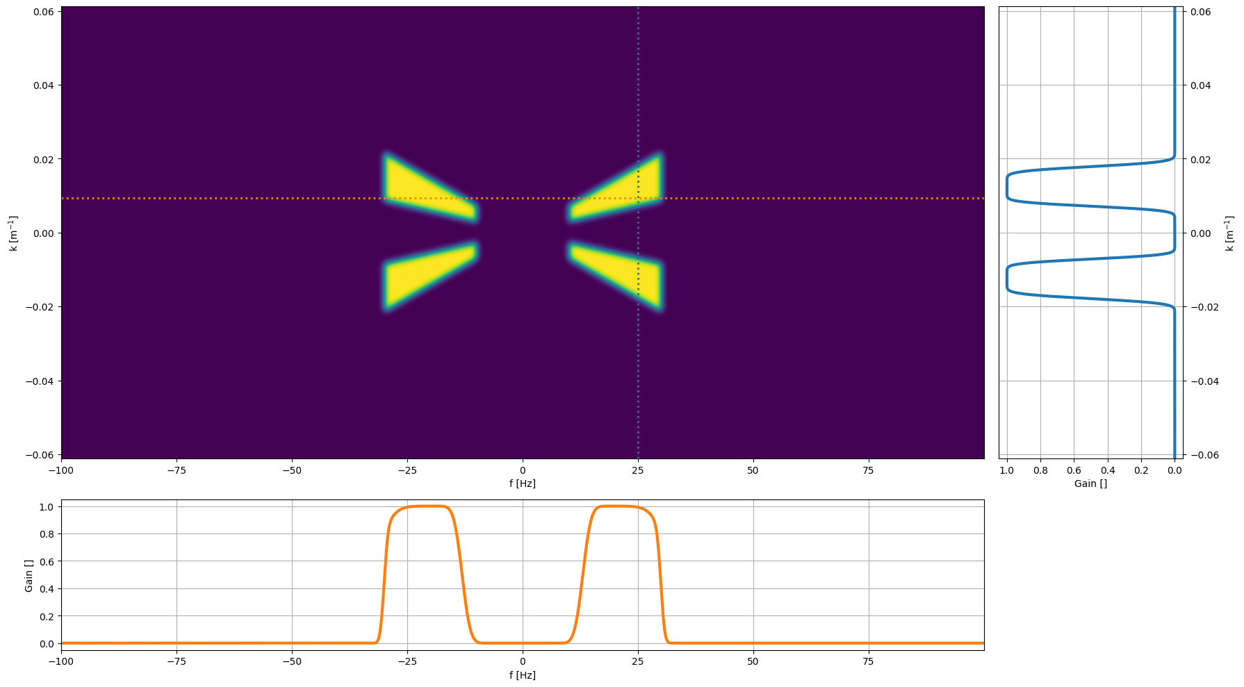
The size of the sparse filter is 0.0359 Gib
The size of the dense filter is 0.49 Gib
The compression ratio is 13.73 (92.7 %)

Warning

The output of the above cell shows the difference between a sparse and a dense filter matrix. The values will depend on the selected channels and the parameters of the filter. If not needed, comment out the line dw.tools.disp_comprate(fk_filter) to avoid the output.

png

Spatio-spectral representation¶

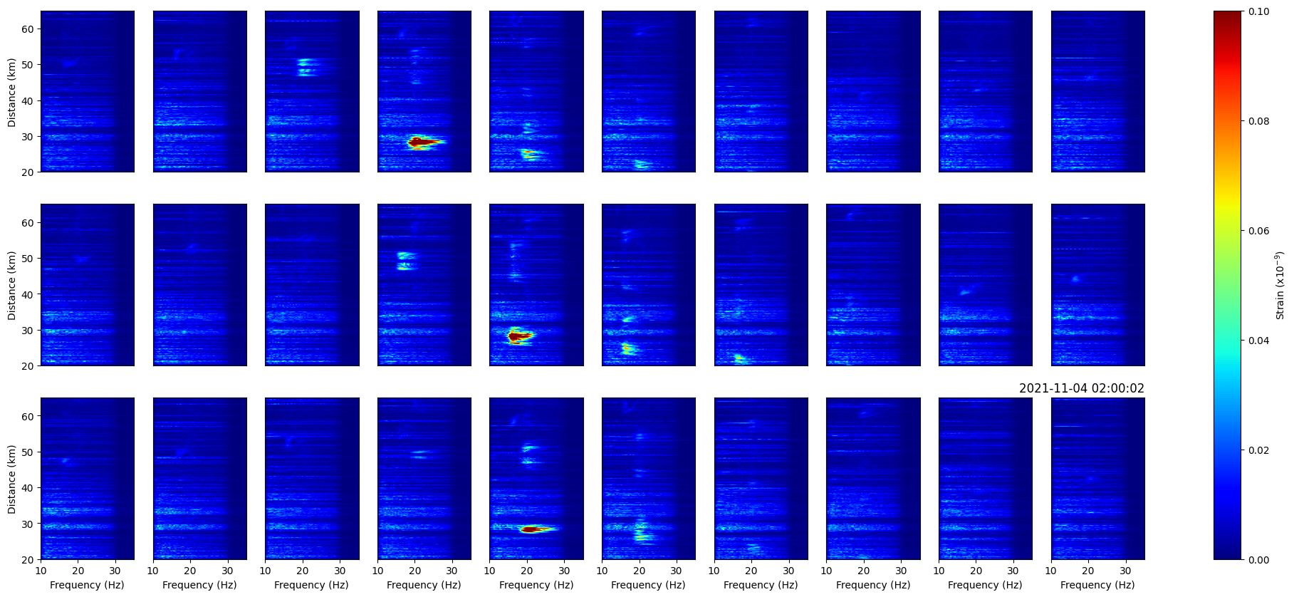
Different features are considered to identify the calling species such as the rhythmic or inter-call intervals, the intensity or received levels, the contours in the time-frequency domain. However, the decisive characteristics to classify baleen whales is the spectral content of the signal. We therefore propose a spatio-spectral representation of the DAS recordings or f-x plot to show the spectral signature and its evolution against the distance.

In the following example, the FFT is applied to each channel of 2-s clips of the spatio-temporal DAS data. The clip duration is specified by the parameter win_s

# Spatio-spectral plot
dw.plot.plot_fx(trf_fk, dist, fs, title_time_info=fileBeginTimeUTC, win_s=2,
                nfft=512,  f_min=10, f_max=35, fig_size=(25, 10), 
                v_min = 0, v_max = 0.1)

png

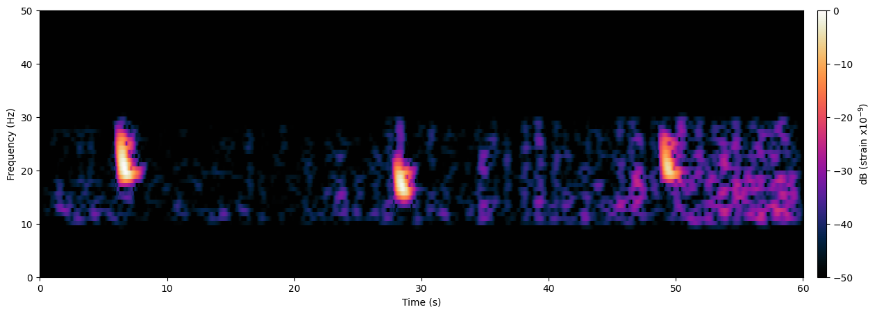
Select channel and display its spectrogram and associated audio¶

from IPython.display import Audio, display

# read one channel only as audio
selected_chan = 28000 # (m)
idx = (np.abs(dist - selected_chan)).argmin()

# Spectrogram
p,tt,ff = dw.dsp.get_spectrogram(trf_fk[idx,:], fs, nfft=256, overlap_pct=0.95)
dw.plot.plot_spectrogram(p, tt,ff, f_min = 0, f_max = 50, v_min=-50)
display(Audio(data=trf_fk[idx,:], rate=fs*5))

png

# read one channel only as audio
selected_chan = 50000 # (m)
idx = (np.abs(dist - selected_chan)).argmin()

# Spectrogram
p,tt,ff = dw.dsp.get_spectrogram(trf_fk[idx,:], fs, nfft=256, overlap_pct=0.9)
dw.plot.plot_spectrogram(p, tt,ff, f_min = 0, f_max = 50, v_min=-30)
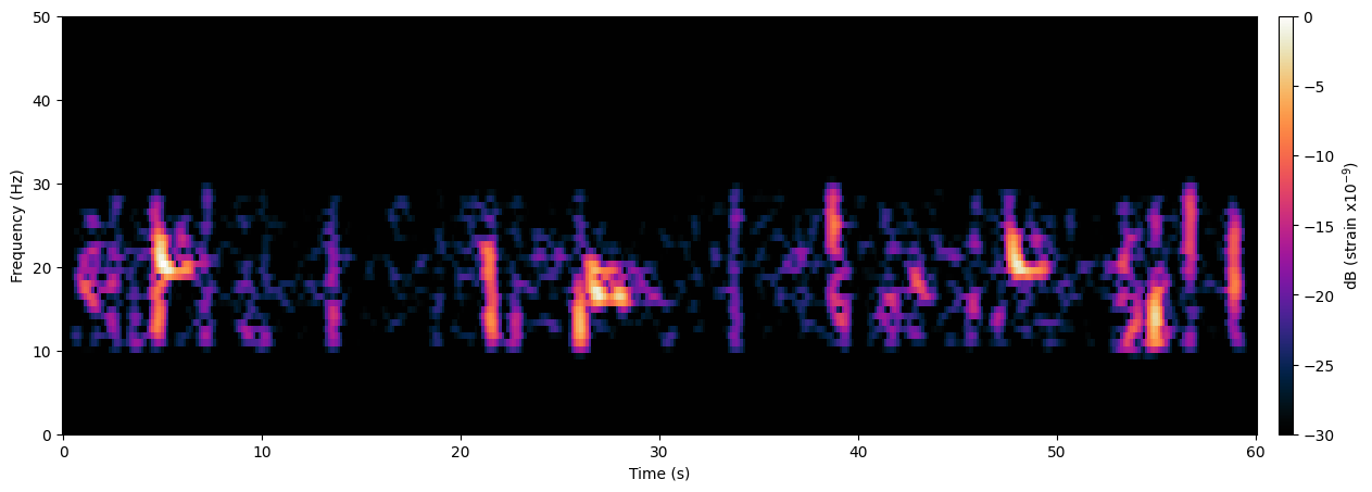
Audio(data=trf_fk[idx,:], rate=fs*5)

png